Courses/Computer Science/CPSC 203/CPSC 203 Template/Fall 2009 Teaching Assistants/F09 Thomas Burt/Lab 2
Contents
Lab 2
Begin by opening the "Movies Spreadsheet" above.
Tasks
- Custom calculations
- If/Then/Else Expressions
- Lookup Functions
- Pivot Tables
Custom Calculations
Excel allows us to input own own expressions to be used along side of the built-in functions. The language for these expressions is much like regular algebra, +, -, *, /, parenthesis all do what you would expect.
Create a new column called "Gross Per Ticket" to the right of "Tickets Sold". We're going to write an expression to calculate how much money was made per ticket.
Click in the first row of the new column, and type the following:
=(g2 / h2)
and press return. You can AutoFill the the rest of the columns, Excel should use the data from the appropriate rows.
If/Then/Else Expressions
These expressions are one of the most common used. They contain three parts:
- conditional
- true value
- false value
The conditional is an expression that returns true or false. Numeric expressions sometimes will consider 0 (or anything less than 1) to be false, and 1 (and anything greater than 1) to be true. Usually, a comparison operator such as =, <, <=, >, >= will be used, although many functions also return true or false values.
First, we're going to summarize which movies are okay for young children. Type the following into column J:
=IF(F2="R", "not good", "okay")
Next, we'll use nested if statements to categorize our data into three sections: "blockbusters", "success", and "flops".
We can use the If/Then/Else expression to do so.
Type the following into column K:
=IF( G2 > 290000000, "blockbuster", IF(G2 < 190000000, "flop", "success"))
Use AutoFill to populate the entire table with these statements.
Lookup Functions
We're going to use a "Lookup Table" to do the same thing we just did with the if statements. Type the following into the second row of a new column:
=LOOKUP(G2,$B$18:$B$20,$C$18:$C$20)
We need to use the "$" in front of the because we don't want AutoFill to try and change the cells we are using for the lookup. The "G2" cell does need to change as usual. Now, use AutoFill to populate the rest of the column with these values.
- Note that the numeric data for the lookup area of the spreadsheet needed to be in ascending order.
Pivot Tables
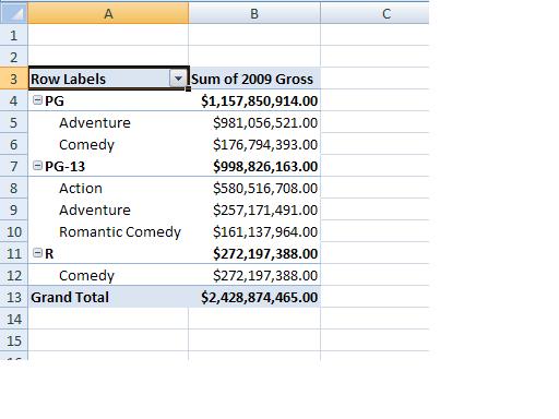
First, select the entire table by clicking in the top left cell and dragging to the bottom right cell. Include some of the columns we made today, but made sure they have column headers or they won't show up as options for our pivot columns.
Now, select the "Insert" tab near the tops of the page. Click the "Pivot Table" icon and press "OK".
A new spreadsheet will open. Along the right hand side of the screen is the "PivotTable field list". Click on some of the fields. The order in which they are clicked will determine how the report is generated.
