Courses/Computer Science/CPSC 203/CPSC 203 Template/Labs Template/Week 1 - Lab 2: Complex Calculations, If-Then Statements, and Pivot Tables

Introduction

Today's tutorial continues to build on the basics of spreadsheets, introduced in the last tutorial. After completing this module, you should be comfortable in demonstrating the following skills:

• doing a custom calculation using a formula (possibly in several steps)
• using a nested If... Then statement to define classes
• summarizing data in a Pivot table
• using a Lookup table to define classes

Do a custom calculation using a formula (possibly in several steps)

In addition to the provided formulas in Excel, custom calculation can also be performed. A custom calculation use the data associated with cells in a single worksheet, or across multiple worksheets. A custom calculation is specified in the function toolbar.

• A cell, in the same worksheet, is referenced by column and row, e.g. F11.
• A cell in a different worksheet is referenced by sheet name, exclamation point, and cell reference, e.g. Sheet2!A1
• The following steps show how to perform a custom calculation:
  • Step 1
    • Select the cell in which you would like the evaluation of the custom calculation to be displayed
  • Step 2
    • In the Function toolbar, enter the custom calculation by starting with the equals symbol '='.
  • Step 3
    • After entering the custom calculation, press the 'enter' key to evaluate the function. The result will appear in the cell that was originally selected.
• A custom calculation can also include functions which are bundled with Excel.

Use a nested If... Then statement to define classes

• An If-Then statement answers the question "is this true or false?" and then performs a corresponding action.
• An If-Then statement consists of three parts: logical test, true statement, and false statement.
  • where the if-part refers to the logical test, and the then-part refers to either the true statement or false statement
• As with performing a custom calculation, and If-Then statement is entered in the Function toolbar.
• The syntax of an If-Then statement in Excel is: =IF(<logical statement>, <true statement>, <false statement>)
  • where the items in angle brackets are replaced by their proper statements/values
• A statement can correspond to a number, or a string of characters by using double quotation marks (e.g. "yes", "true", "evaluation if false", etc.)
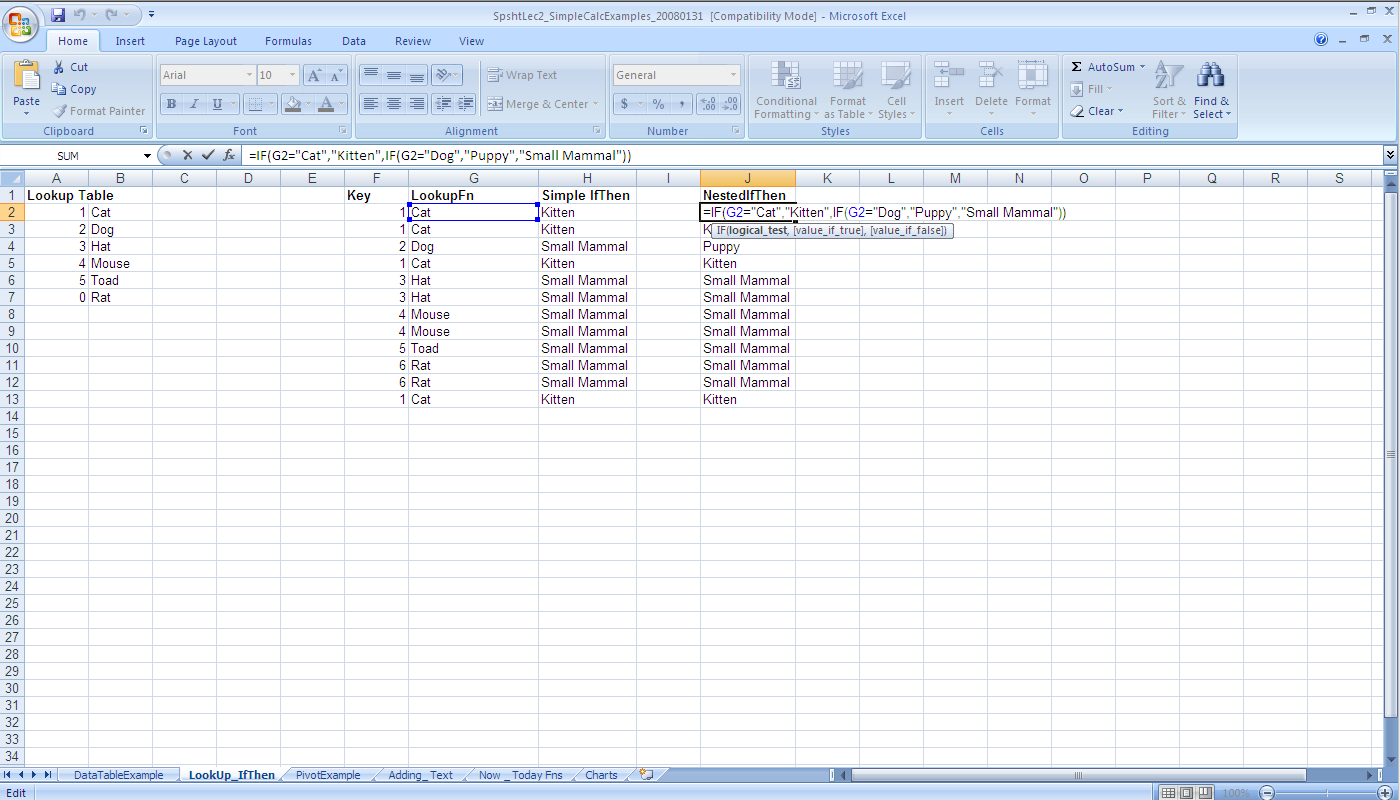
• An example If-Then statement can be found in the following spreadsheet.
• A nested If-Then statement can be created, if the true statement and/or false statement consists of another If-Then statement.
  • See the following spreadsheet for an example.
  • In nested If-Then statements, evaluations of inner-most statements occur first, and their evaluations are propagated to the outer-most statements.
    • See the following example

Summarize data in a Pivot table

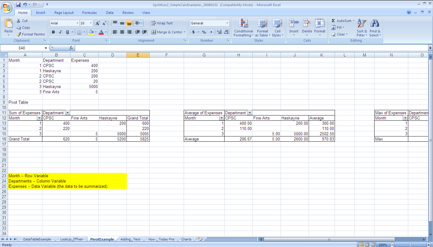
Large amounts of data can quickly accumulate in a spreadsheet. Pivot tables provide a mechanism to summarize data, and as a result, makes it easier to analyze and present data. Perform the following steps to create a Pivot table

• Step 1: select a range of cells, or table. Important Note: make sure the range of cells have column headings.
• Step 2: select the 'PivotTable' icon under the 'Tables' contextual menu as part of 'Insert' in the main toolbar.
• Step 3: in the new panel that appears make sure that the selected range of cells or table is correct, and specify the destination of the Pivot table
• Step 4: a new Pivot table is created. Added to the main toolbar is 'PivotTable Tools' (along with its associated contextual menus), when the Pivot table is selected. As well, a 'PivotTable Field List' panel also appears when the Pivot table is selected. Use the options in the contextual menus and panel to format the Pivot table and present the data in an appropriate manner.

For further information regrading Pivot tables, please refer to:

• http://office.microsoft.com/en-us/excel/CH100648481033.aspx

Use a Lookup table to define classes

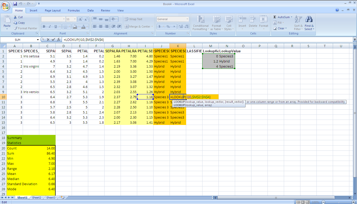
Lookup functions can be used to find values (data) in a data table, essentially answers to questions. Several lookup functions are provided in Excel. A list of lookup functions can be found here:

• http://office.microsoft.com/en-us/excel/HP100791881033.aspx?pid=CH100645331033

We will go through an example using the Lookup and VLOOKUP functions.

• The syntax for the Lookup function is either
  • =Lookup(lookup_value, lookup_vector, [result_vector])
    • lookup_value is the value to search for in the lookup_range
    • lookup_vector is a single row or single column of data that is sorted in ascending order (the Lookup function searches for value in this range)
    • [result_vector] is a single row or single column of data that is the same size as the lookup_range; the Lookup function searches for the value in the lookup_range and returns the value from the same position in the result_range
  • =Lookup(lookup_value, array)
    • lookup_value is the value to search for in the array (values must be in ascending order)
    • array is an array of values that contains both the values to search for and return

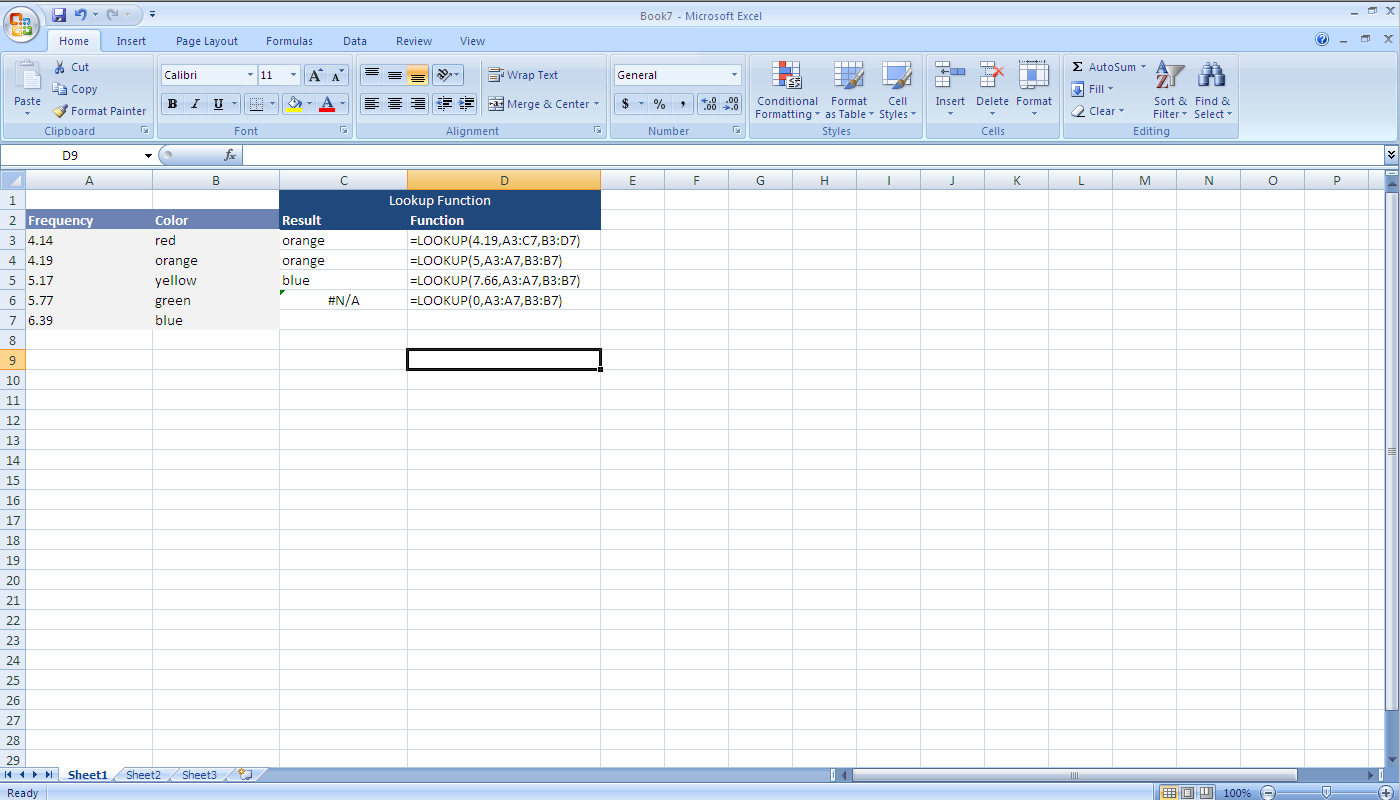
It is important to understand how Excel interprets the cut points. The following example illustrates the three points below, and is based on an example provided in Excel 2007 Help (Excel > Function Reference > Lookup).

• In the case of equality (=), a match is found, and its corresponding value is returned; the first example where 4.19 is found in column A and the corresponding value in column B is returned, orange
• In the case of greater than (>), the next smallest value is found, and its corresponding value is returned; the second example where 5.00 is not found and instead 4.19 is found in column A and the corresponding value in column B is returned, orange
• in the case of less than (<), if the value is less than any value, N/A is returned; the fourth example where 0 is less than every number in column A, and as a result, N/A is returned

The VLOOKUP function looks in the first column of a data table and finds the corresponding value in the row.

• The syntax for the VLOOKUP function is: =VLOOKUP(lookup_value, table_array, col_index_num, [range_lookup])
  • lookup_value corresponds to the value being searched for in the first column
  • table_array corresponds to the range of cells
  • col_index corresponds to the column that represents the data of interest
  • [range_lookup] corresponds to finding an exact match or an approximate match. Important Note: this is an optional argument, but it is best to use the value FALSE to specify that that the data is not in ascending order.

Using Absolute References in Lookup Function

Based on http://office.microsoft.com/en-us/excel/HA102874681033.aspx

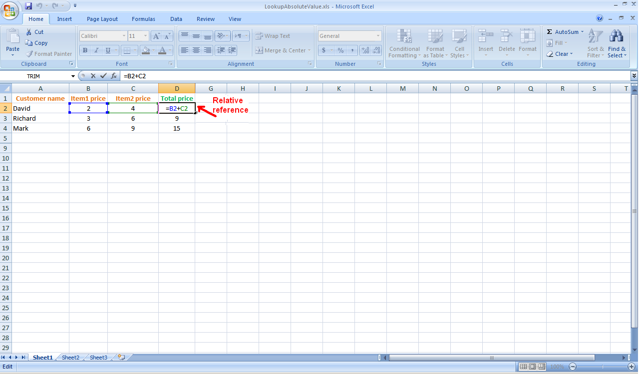
• A relative cell reference adjusts to its new location when the formula is copied and pasted. For example, the figure below shows the prices of the items bought by three customers at a store. The total amount to pay by each customer is in the “Total price” column. For instance, the summation formula is B2+C2 (for the values 2 and 4) for the element in cell D2. If we drag the equation through the rest of column D, the formula will be updated to reflect the corresponding values in the same row. For instance, if we go to cell D4, we will find that the formula is automatically updated to be B4+C4 so that it would sum the values 6 and 9.

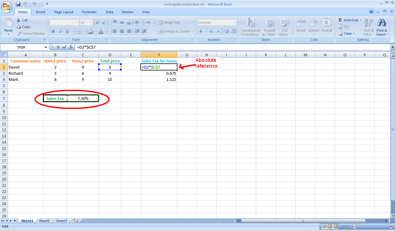
• An absolute cell reference does not change, even when the formula is copied and pasted elsewhere. An absolute reference is specified with two dollar signs, where the first dollar sign precedes the column and the second precedes the row. For example, in the figure below, the sales tax percentage for all the items bought by the different customers is added in cell C7. To calculate the sales tax for every customer’s items, all the different items should reference the same Sales tax percentage value. Hence, the sales tax is calculated for the first customer using the absolute reference for the Sales Tax (as $C$7), and then the formula is copied to the rest of the rows while keeping the same absolute value.

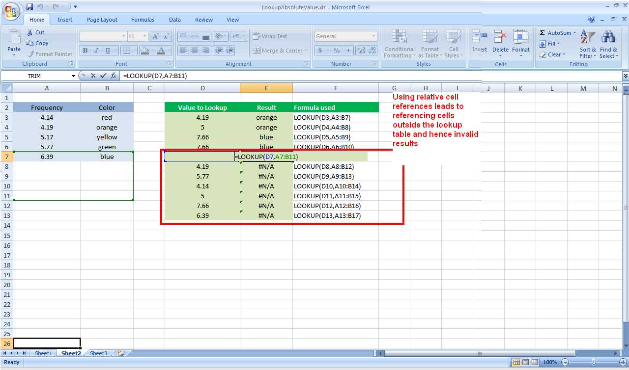
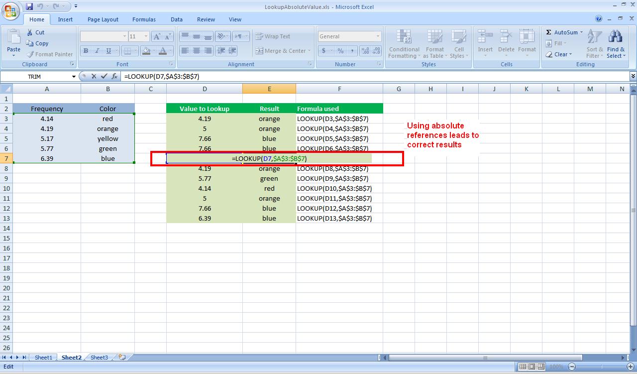
• When referencing lookup tables, absolute values should be used, or else invalid values will be displayed if the lookup table is smaller than the values to lookup. In the figure below, using relative references for the lookup table leads to referring to blank fields. For instance the formula lookup(D7, A7:B11) references rows 8 to 11 which are blank rows. In the following figure, the problem is fixed by using absolute references to the lookup table values.

Invalid lookup function

Valid lookup function