Courses/Computer Science/CPSC 203/CPSC 203 Template/Labs Template/Week 3 - Lab 1: Analysis and Forecasting

Notes

• These notes are for development of the module only.

FILES

You can download the example file for this lab from here: Media:Analysis example.xls

Additional Resources

• Take a look at the textbook, "Fluency" Pages 399-401 which has a loan payment example. It uses a function called PMT.
• Take a look at the textbook, "Fluency" Pages 396-399 which has a discounting example.

Introduction

You will work through an example of applying Excel's forecasting features to perform a compound interest calculation. The compound interest is the amount of money earned on a deposit during a period of time. It can be calculated using the following formula:

 P= C (1 + r/n)^nt

where

• P = future value
• C = initial deposit
• r = interest rate (expressed as a fraction e.g. 0.06 = 6%)
• n = # of times per year interest is compounded
• t = number of years invested.

Skills

After completing this module, you should be conformable in demonstrating the following skills:

• forecasting

Analysis

• Two spreadsheets on Blackboard
  • AnalysisExamples_Su07ClassSurveySimpleAnalysisIdeas.xls
  • AnalysisExamples_PresidentsDataAndAnalysis_4_20080306.xls
• Items to show/demonstrate
  • Summaries
  • Scores
  • Models (with assumptions)

Forecasting

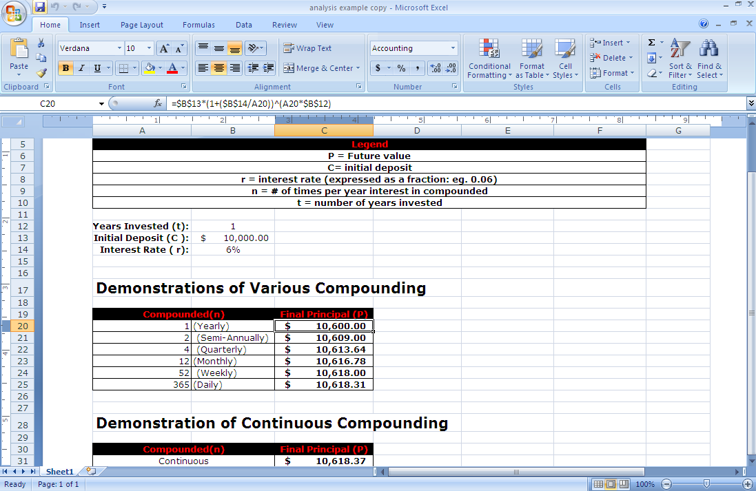
You should setup your excel document so that it is easy to read and make modifications. Use the example layout as depicted below: This layout makes it easy to look up parts of the Compound Interest Formula as well as makes it easy to adjust the formula to try out new scenarios. Format your cells so that the correct number representation is shown, e.g. Initial Deposit is using the Currency Formatting while Interest Rate is using the Percentage Formatting.

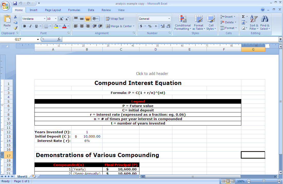
Create a legend for your formula, and the 3 sections for Years Invested, Initial Deposit, and Interest Rate. Afterwords create a table that will display the compounded times available and the final principal which will tell you how much money you earn given the compound frequency and the interest rate available. We will determine the Final Principal using the formula stated above.

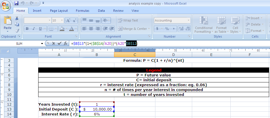
For the Final Principal field, you will notice the formula used in the formula bar. =$B$13*(1+($B$14/A20))^(A20*$B$12)

What do these values correspond to?

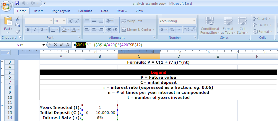
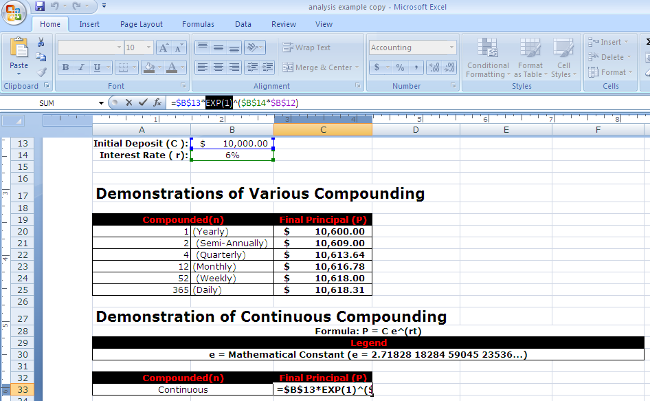
Let us take a step by step look at how this formula was created and what these values correspond to. As you can see in the picture depicted below, the highlighted $B$13 in the formula refers to cell B13 which is the value for Initial Deposit (C). The dollar signs ($) are used because we want to keep this cell constant where ever we use the formula, we always want it to refer to B13 to get the value for Initial Deposit. This also makes it easy for you to change the initial deposit amount and experiment will different values without having to modify lots of different cells.

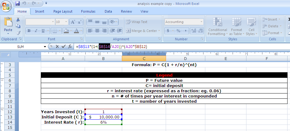
Continuing on to the next variable in the formula, the highlighted $B$14 in the formula refers to cell B13 which is the value for the Interest Rate (r). Again the dollar signs ($) are used because we want to keep this cell constant where ever we use the formula.

Our last variable to examine in the formula for now is $B$12 which refers to cell B12 the number of years invested (t). Again the dollar signs ($) are used because we want to keep this cell constant where ever we use the formula.

It should start look more obvious that the formula in the formula bar is matching the one given earlier of P = C(1 +r/n)^(nt).

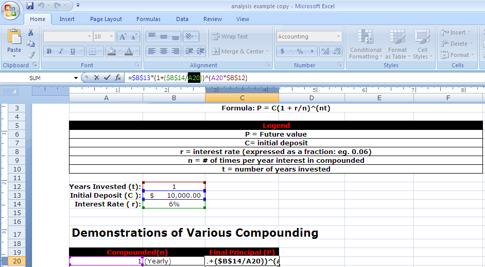
So that leaves us with A20 in the formula, A20 refers to the number of times per year that interest is compounded. Here we have created a table with lots of different options for compounding events which include: Yearly, Monthly, Quarterly, Daily, etc. NOTE: we refer to A20 which contains a number and not B21 as it just contains text. Our formula requires numbers to be used.

Looking at the next compounding event, Semi-Anually, you will see that in the formula A20 becomes A21. Meanwhile all the other variables in the formula have not changed because of course we are using the dollar signs ($) to keep those values constant. If you examine the remaining compounding events you will see the same thing occurring, A21 becomes A22, A22 becomes A23 to reflect the changing compounding event.

[Image:Forecast8.png]]

So what about Continuous Compounding Interest? This type of calculation requires a slightly different but similar formula but is very simple for you to calculate. First we need to introduce the new formula and a new variable.

P = C e^(rt)

So e is a mathematical constant that is used for this formula, to which you can refer in calculation using EXP(1).

So here is the e mathematical constant variable used in the formula.

Sorting

This section is based on Microsoft Office 2007 Help.

Microsoft Excel allows you to sort your data whether it is textual, or numerical.

Sorting Textual Data

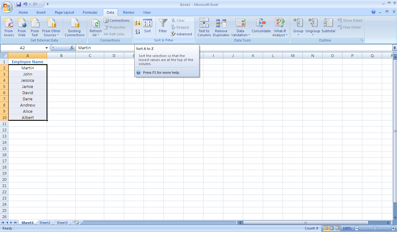
Given the list of names of employees in a company, you can sort those names by selecting the range of values you want to sort, and then selecting how to sort them from the Data tab (see the following example).

On the Data tab, in the Sort & Filter group:

• To sort in ascending alphanumeric order, click Sort A to Z.
• To sort in descending alphanumeric order, click Sort Z to A.

Names before sorting

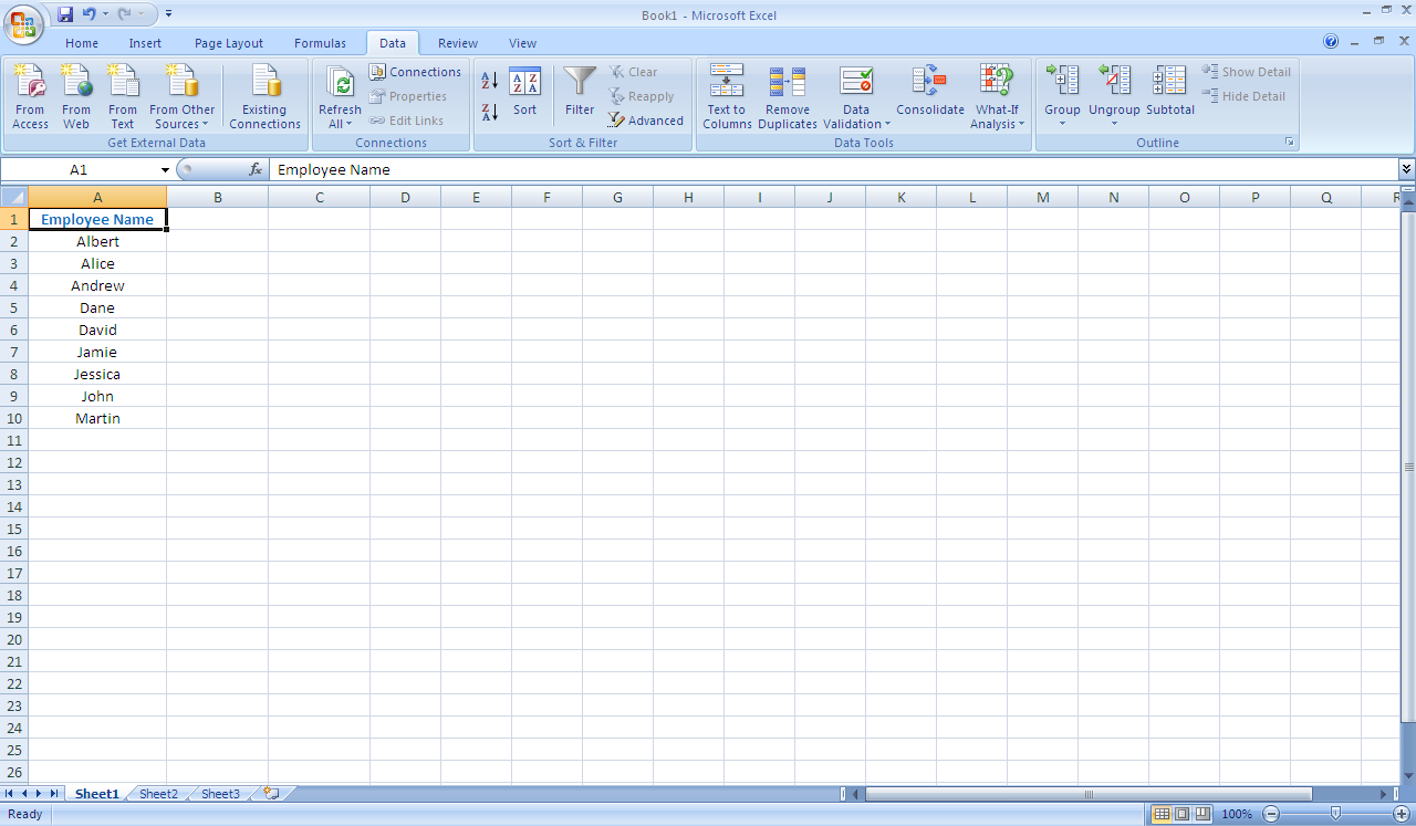
Names after sorting

Sorting Numerical Data

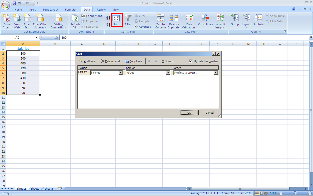
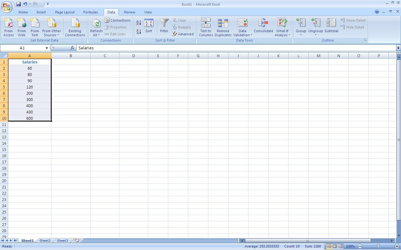
Similar to sorting textual data, you can sort numerical data by selecting the range of values you want to sort, and then selecting how to sort them from the Data tab (see the following example).

Salaries before sorting

Salaries after sorting

Sorting by more than one column

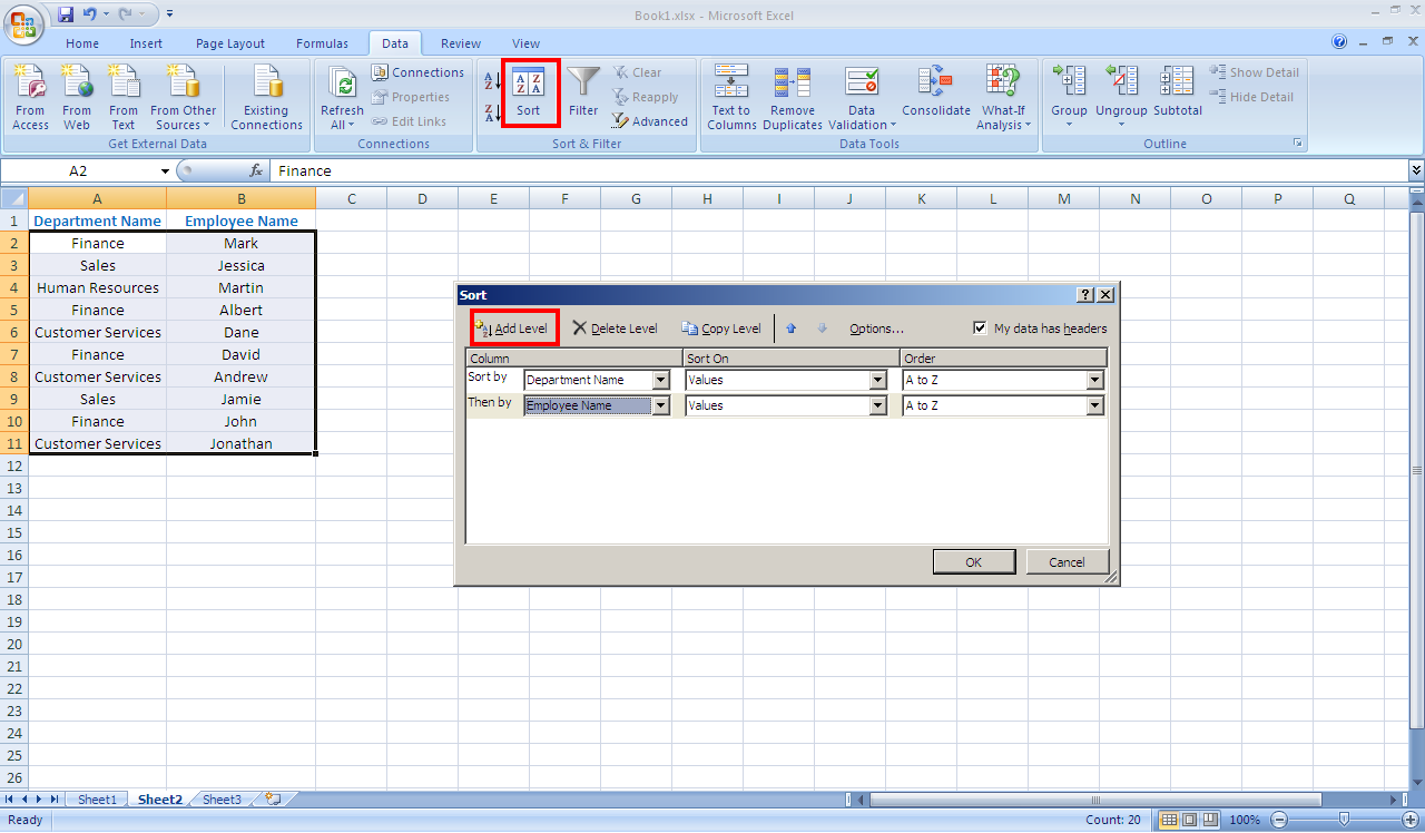
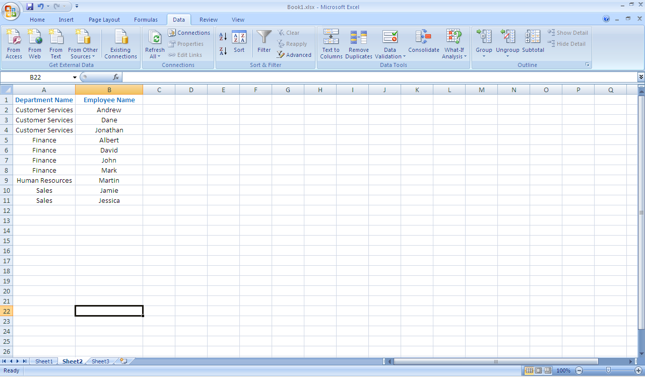
You can sort by more than one column. For example, the figure below shows the names of employees working in several departments. We would like to sort by Department (to group all the employees in the same department), and then sort by name (to alphabetically sort the names of the employees of every department).

To sort by several columns, do the following:

• Select the "Department Name" column, and the "Employee Name" column
• On the Data tab, in the "Sort and Filter" group, click "Sort"
• Select the first column that you want to sort by (the "Department Name" column), and select how you want to sort the data (On values from A to Z)
• Add a second sorting level for the "Employee Name" column, and select how you want to sort the data (On values from A to Z)

Departments and Employees names before Sorting

Departments and Employees names after Sorting

Filtering

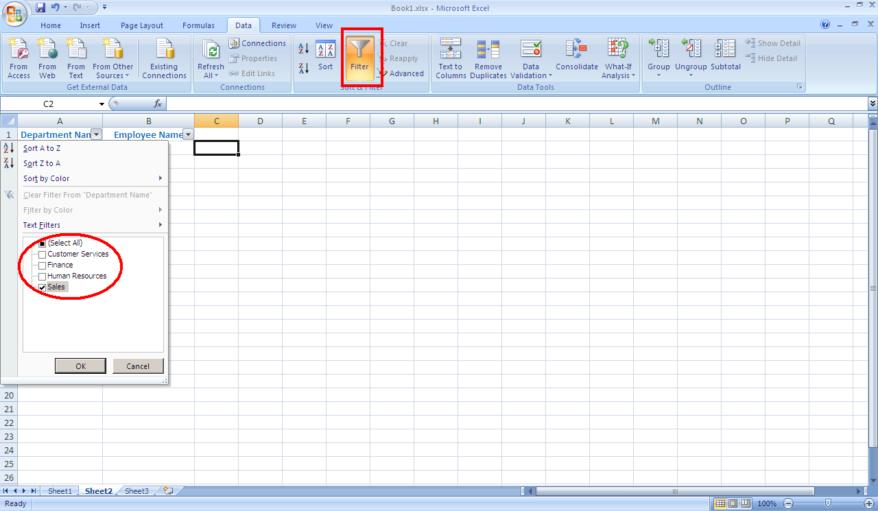
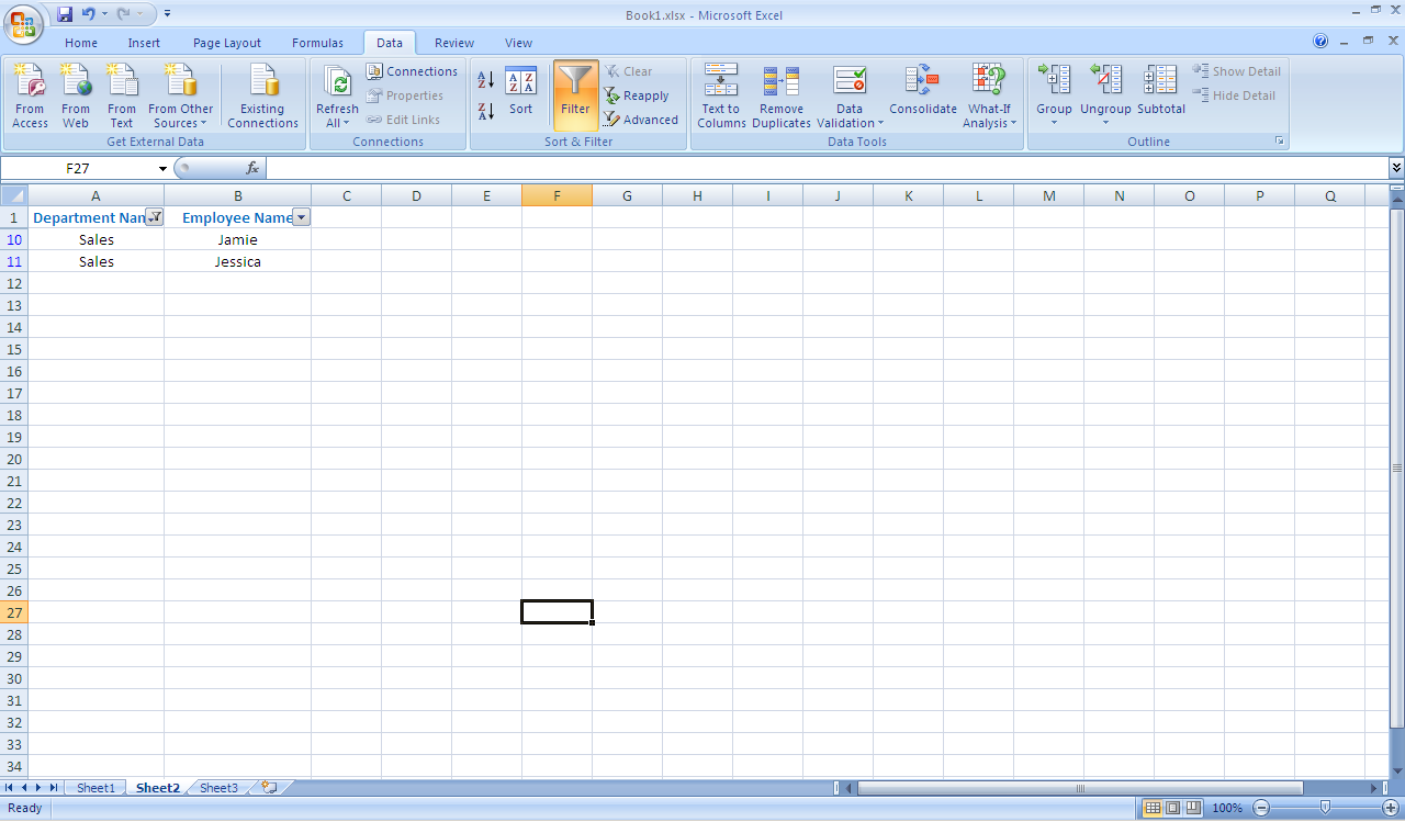
Filters allow you to display only a portion of the data that matches a certain criteria. Given the list of departments names, and employees names in those department, you can make filters to display information for only the "Sales department. This can be done by selecting the data you want to filter, and clicking on the "Filter" button in the Data tab.

Filtering the departments names

Only information for the "Sales department is displayed.

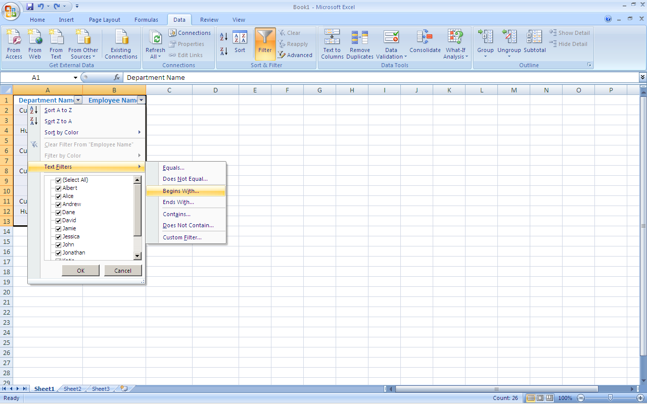
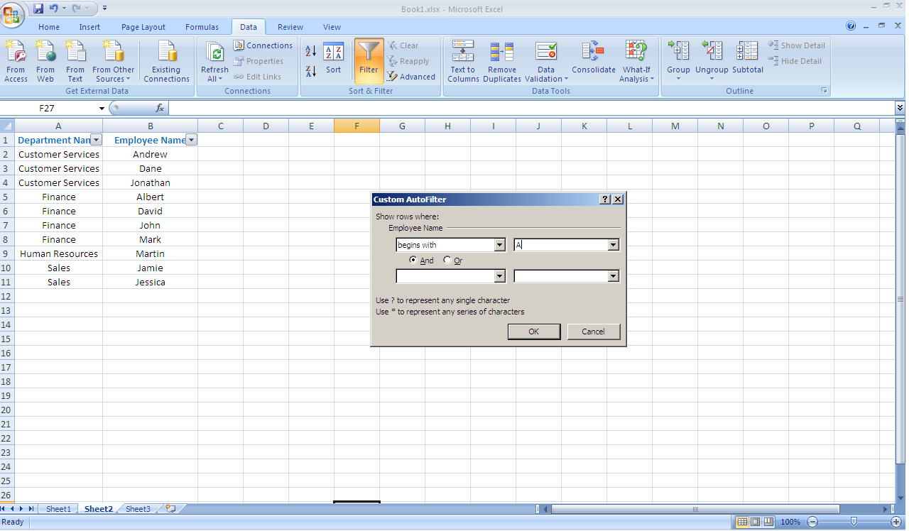
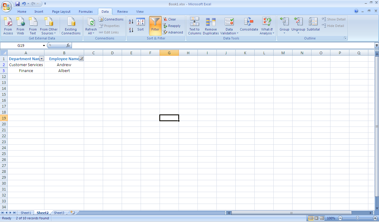
Customized Filters You can also filter based on some criteria that you enter. For example, lets say you want to display only the names of employees that start with an "A". This can be done by opening the "Employee names" column filter, and selecting the "Begins with" menu item from the "Text Filters", and specifying that the names to be displayed should start with an "A".

Step 1: Opening the "Text Filter"

Step 2: Specifying that the names should begin with an "A"

Result: Only the names starting with an "A" are displayed

Filtering for unique values

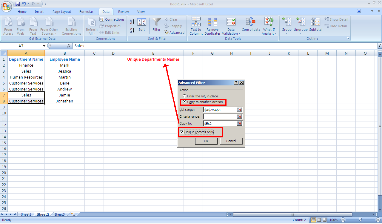
You can filter a list of values to show only the unique values in that list. This can be done using the "Advanced Filter" option. For example, lets get the list of unique departments names from the table shown below. This can be done by selecting the list of departments, and clicking the "Advanced Filter" button as shown below.

Step1: Using filters to copy the unique values to another cell

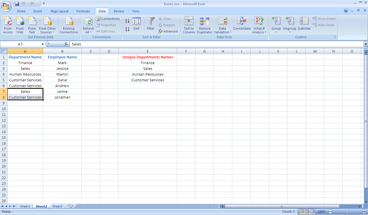
Result: The unique departments names copied to a new column